自回归模型:MAR
原文链接:https://arxiv.org/pdf/2406.11838
参考资料:何恺明:Autoregressive Image Generation without Vector Quantization.
摘要
Conventional wisdom holds that autoregressive models for image generation are typically accompanied by vector-quantized tokens. We observe that while a discrete-valued space can facilitate representing a categorical distribution, it is not a necessity for autoregressive modeling. In this work, we propose to model the per-token probability distribution using a diffusion procedure, which allows us to apply autoregressive models in a continuous-valued space. Rather than using categorical cross-entropy loss, we define a Diffusion Loss function to model the per-token probability. This approach eliminates the need for discrete-valued tokenizers. We evaluate its effectiveness across a wide range of cases, including standard autoregressive models and generalized masked autoregressive (MAR) variants. By removing vector quantization, our image generator achieves strong results while enjoying the speed advantage of sequence modeling. We hope this work will motivate the use of autoregressive generation in other continuous-valued domains and applications.
研究动机
由于语言先天的离散性质,在自然语言领域的自回归模型都是在离散的隐空间中学习数据的概率分布。因此,当自回归模型推广到连续的数据空间(如图像生成)进行发展时,研究人员将主要的精力放在了如何更有效地将连续数据离散化上,如 VQGAN、VQVAE、VAR、MaskGIT 等。
然而,本文作者从 Autoregressive 模型的性质本身(即根据先前的 token 预测下一个 token)出发进行思考,产生了自回归模型是否有必要与向量量化(Vector Quantization)表示相结合的疑问,作者发现,自回归生成模型与 token 是离散表示的还是连续表示的并没有关系,真正需要解决的问题是如何对每个 token 的概率分布进行建模,同时该概率分布可以通过损失函数来学习和约束(训练),并用于从中进行采样(生成)。
主要方法与实现
本文提出的模型融合了目前图像生成领域的三大主流范式的思想,分别为自回归生成、掩码生成以及扩散生成:
- 模型首先根据自回归模型性质为每个 token 生成条件向量(conditional vector)
- 之后使用扩散过程建模每个 token 的概率分布
- 最后结合掩码生成的思想加速训练和推理过程
Diffusion Loss
具体而言,如下图所示,假设连续值向量 ,是当前位置要预测的 token。自回归模型在这个位置产生一个条件向量 。
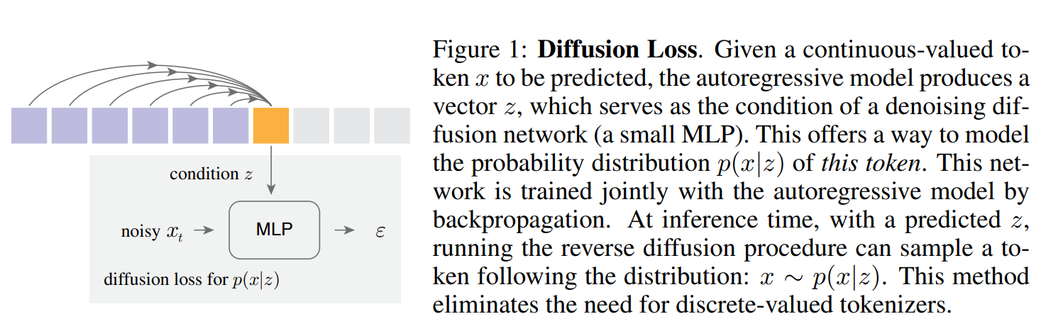
本文使用 Diffusion Loss 根据 对 建模概率分布 。
其中:
-
是从 采样的噪声向量
-
,其中 定义了一个 noise schedule
-
是 noise schedule 的时间步
-
噪声预测网络 由参数 控制,是一个小型 MLP 网络, 表示此网络将 作为输入,并且以 和 作为条件。MLP 网络的具体组成如下所示:

对于扩散过程,作者采用了 cosine 函数作为 noise schedule,在训练过程中设定为 1000 步,在推理过程中设定为 100 步。同时,Diffusion Loss 原生支持 CFG 策略。
采样
在推理时,需要从分布 中采样样本。采样是通过逆扩散过程进行的:
这里 是从高斯分布 中采样的, 是时间步 的噪声水平。以 开始,此过程生成一个样本 使得 。
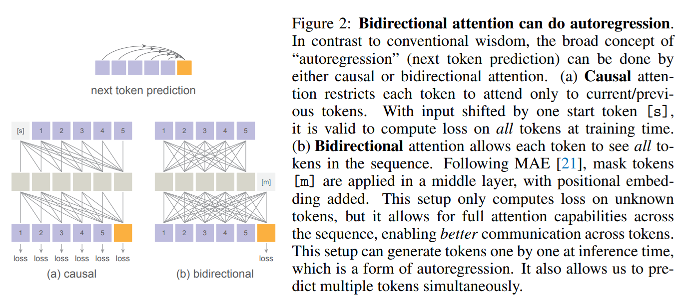
双向注意力机制
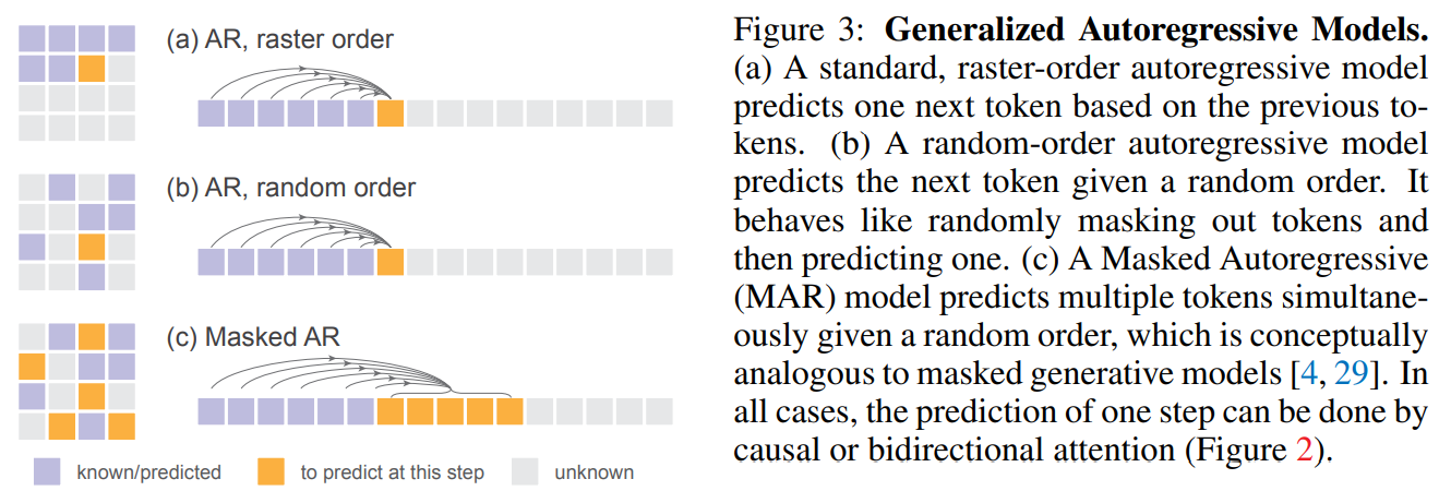
结合掩码生成模型的思想 MAR
本文为了提高生成速度,结合了 MAE 和 MaskGIT 模型的思想,如下图的 b 和 c 所示,将随机顺序生成的思想和每次预测出一个 patch 的 token 的思想加入到本文的模型中。
掩码信息通过位置编码送入 Decoder 中,使模型在以随机顺序预测序列时获取到 token 的位置信息。
实验与结论
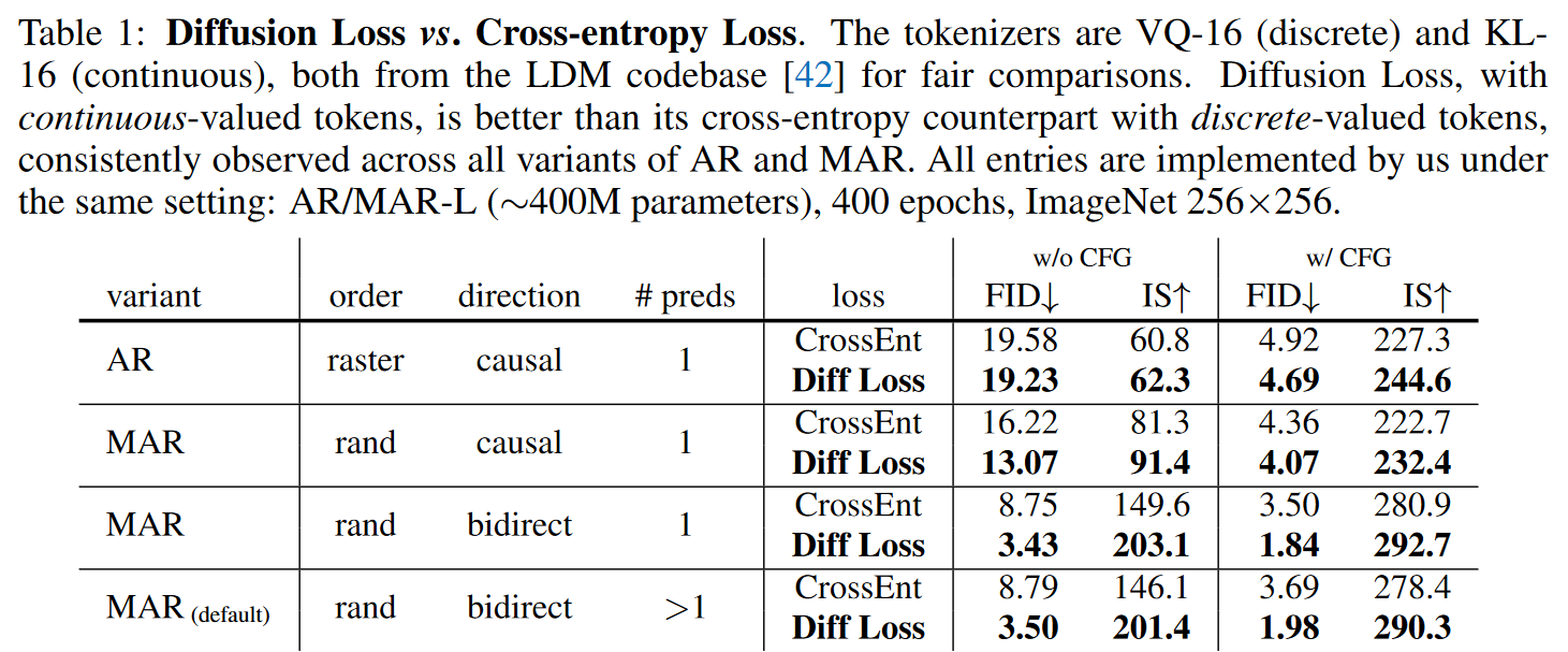
对比离散与连续、单向与双向注意力、逐 token 或逐 patch 预测
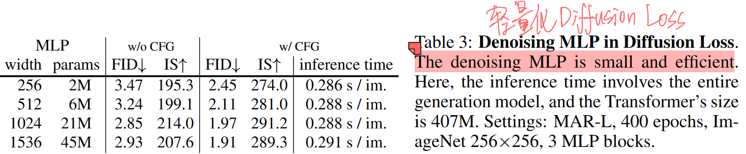
扩散过程 MLP 参数对性能的影响
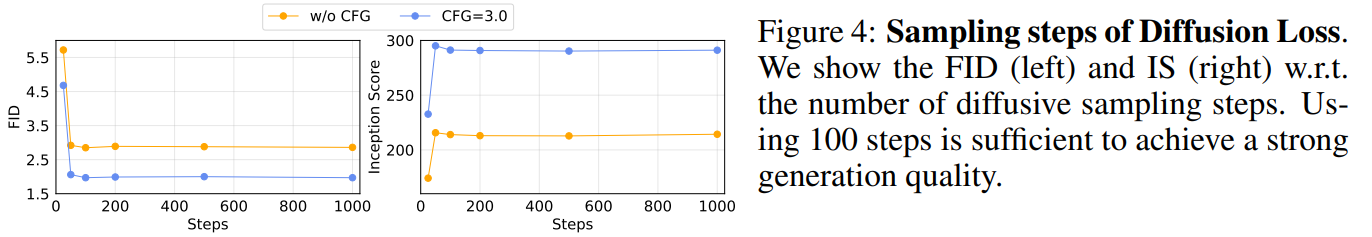
扩散过程采样步数对性能的影响
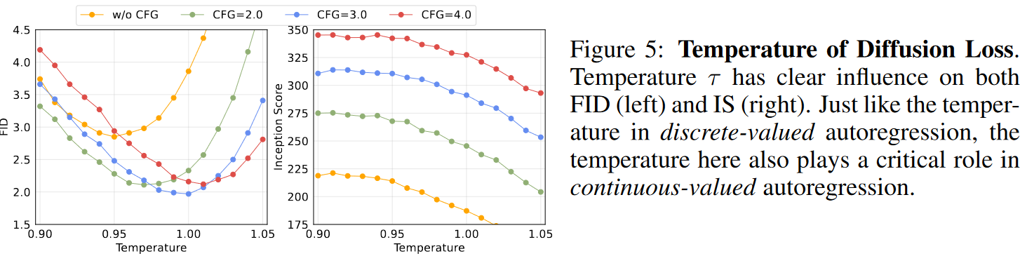
温度对多样性和准确性的控制
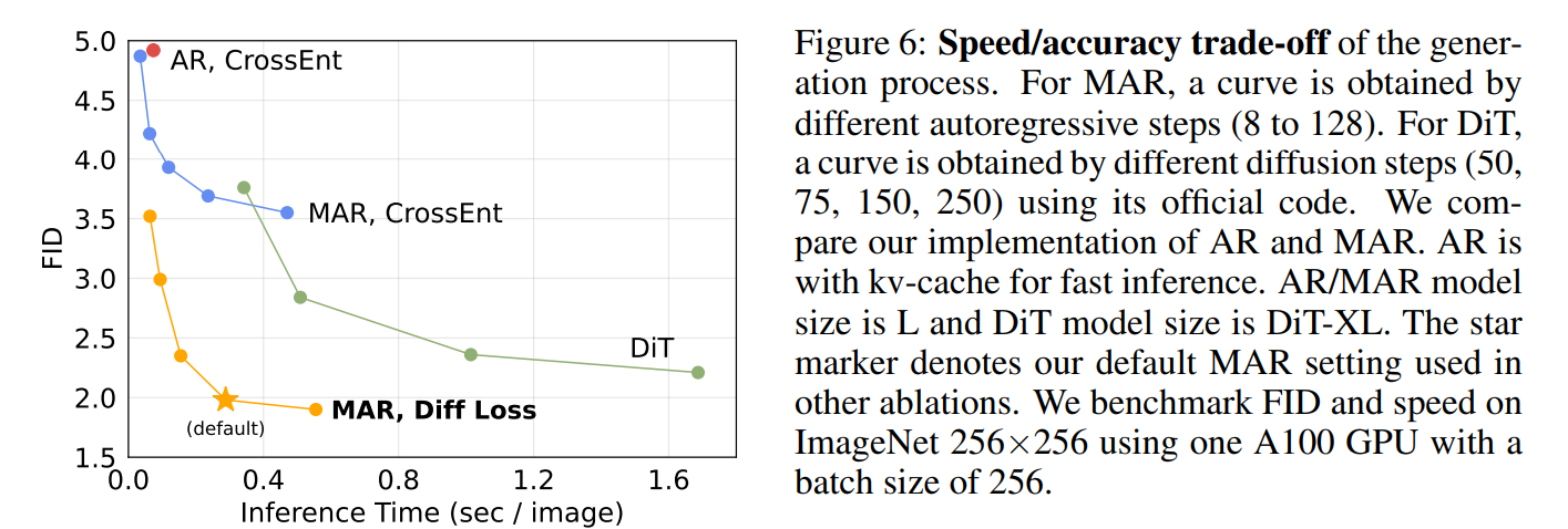
MAR 模型速度与效果的 trade-off
对于 MAR 模型,AR 步数越小,每次预测的一个 patch 的 token 数越��大,速度越快,精度越低,默认设置为 64 步。